I became interested in Machine Learning (particularly text-to-image) since dalle-mega (~June 2022). I have worked to improve the state of ML on Mac (providing fixes and bug reports). Slow Mac performance led me to seek ways to optimize attention and the denoising process. Most of my spare hours since stable-diffusion (~Aug 2022) have been spent developing inference techniques for latent diffusion models. This page journals my progress as a self-taught ML researcher. You can follow my journey on Twitter @Birchlabs. — Alex
Research
Multi-cond guidance
Can we mix multiple denoising predictions? Classifier-free guidance shows that we can mix a cond and uncond.
I tried mixing multiple conditions and even negating them — it turns out I had independently discovered Composable Diffusion.
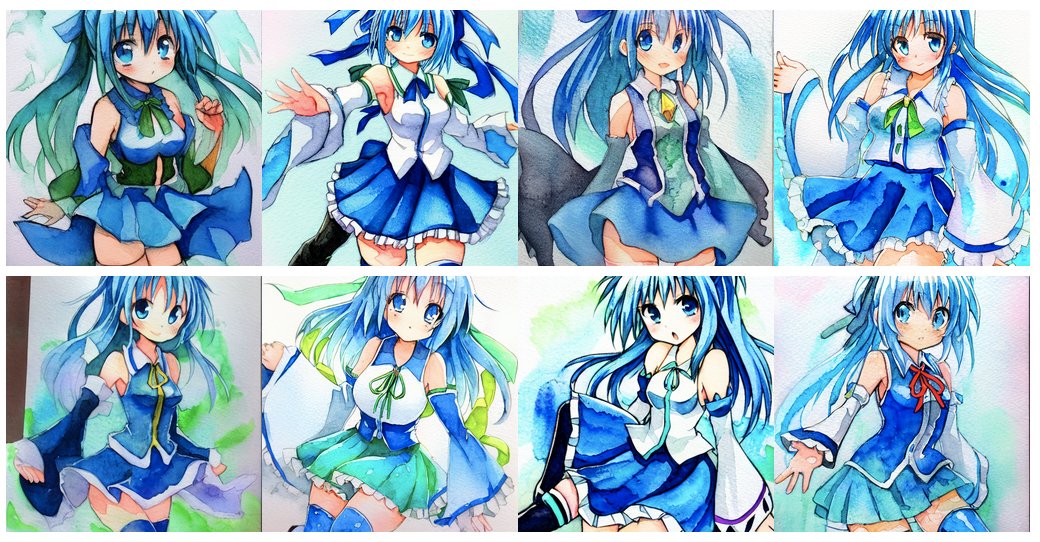
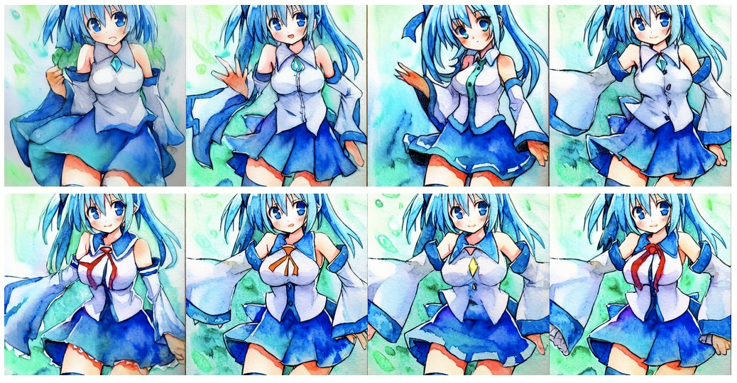
I took the concept further by playing with the ability to tweak the weighting of each denoising prediction. This unlocked a novel way to transition between conditions. Animated, it looks similar to a latent walk but it is a visual rather than semantic traversal.
Approx decode (single linear layer with L2 loss + bias)
Stable-diffusion's latents can — to a good approximation — be decoded to RGB using a simple matrix multiplication.
I took further keturn's idea of "approximate decoding", and erucipe's idea of "learning from blue loss" by training with more discerning loss functions on a larger dataset, and making the network slightly deeper.
Thresholding: heuristic scale (compare n%ile with known-good max)Background
Classifier-free guidance makes diffusion models output images more relevant to text prompting, at the expense of increasing pixel values (potentially going out-of-range). Imagen introduced dynamic thresholding to combat this. But we cannot use this technique on latent diffusion models.
I developed techniques for applying thresholding to latents. This enables us to use higher CFG scales without getting clipped pixel values.
Gated
Unthresholded
Thresholded
CFG scale=30: gated thresholding
Imagen-style thresholding, enabled if latent values exceed arbitrary upper-limit.
We unscale each latent channel (÷0.18215), center each channel on its mean. If any channel has a max exceeding 42: threshold by 99.95%.
This is effective because it tames high/mid sigmas, and ceases once we're past the most of the danger zone (CFG seems to do most of its damage at the start of the schedule — perhaps this indicates that cond and uncond denoising predictions only agree later in the schedule, as noise is removed). We also avoid clamping as aggressively as ±1 (latents are unbounded, so it is damaging to clamp them into ±1 range).
Refer to known-good CFG, scale latents in ratio between our 99.95%iles
We compute a known-good (CFG7.5) output, center channels on means, measure their 99.95%ile latent values. We do the same for our desired (CFG20) output. We divide CFG20's output by the ratio between those 99.95%ile results. We do not apply Imagen-style clamping (latents are unbounded, so it is damaging to clamp them into ±1 range).
Heuristic scaling (compare n%ile with known-good max)
Unthresholded
Thresholded
CFG scale=30: heuristic scaling (n%ile vs max)
Scale latents in ratio between our 99.95%ile and known-good's max
Similar to previous, except extends the dynamic range by considering our "known-good"'s max to also be fine. This retains a bit more subtlety in shadows and highlights.
Decode latents to pixel-space, threshold Imagen-style
Every sampling step: we decode the latents to pixels via VAE, dynthresh them Imagen-style, then re-encode back to latents.
Results in a good dynamic range, but the VAE round-trips are lossy, slow and introduce colour-banding. Could still make sense to do this at the start of the denoising schedule though (combat the worst of the CFG, then resume as normal to fill in final details).
Decode latents, threshold pixels, compare pixels, guide by backprop difference
Similar idea to CLIP guidance. We decode latents to pixels via VAE, dynthresh them Imagen-style. But we don't want to re-encode them (previous technique showed us that VAE roundtrips are lossy). So we compare the unthresholded pixels with our thresholded pixels, compute MSE loss, compute gradient of loss, then apply that difference (scaled by a learning rate) to our original latents.
Results weren't super. Was pretty fiddly, and very few ranges of values did anything other than producing more artifacts.
Decode latents approximately to pixel-space, threshold Imagen-style
Addresses the performance issue of doing a full VAE roundtrip, by distilling a fast encoder and decoder (just a couple of dense layers trained on real VAE inputs/outputs). The approx VAE suffices to do color-space conversion between latents to pixels. It doesn't perform any resampling, which I hoped could help make the roundtrip less lossy. Ultimately it turned out that the approx VAE was too lossy to use on the entire denoising schedule, but we can combat the worst effects of CFG by dynthreshing during high/mid sigmas, then resume without dynthresh to preserve high-frequency details.
CFG scale=30: Threshold in pixel space via approx VAE roundtrip
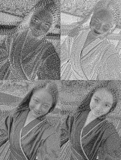
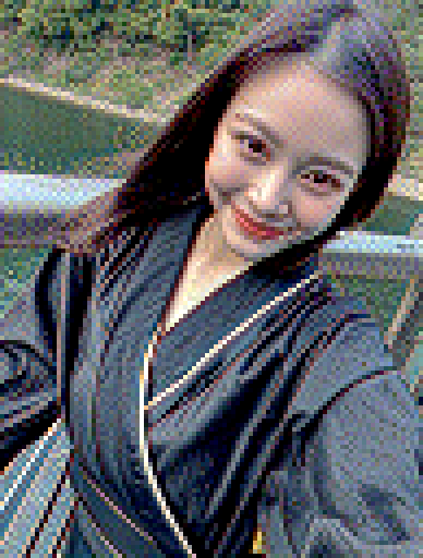
Combating mean drift in CFG
Standard
Centered
Latent values centered on channel means
Stable-diffusion's Unet returns denoised latents with per-channel means of about 0.
This slight deviation from 0 is amplified when CFG is applied. The result then goes back into the Unet, or is decoded by the VAE.
I wondered whether either the Unet or VAE was trained to expect standardized inputs (e.g. mean of 0, and variance of 1).
Prior to applying CFG: I shift the denoised latents to be centered on their per-channel means. The effect was interesting: high-frequency details increase, especially foliage. A bit of grain is created too (perhaps this can be avoided by ceasing the technique late in the denoising process).
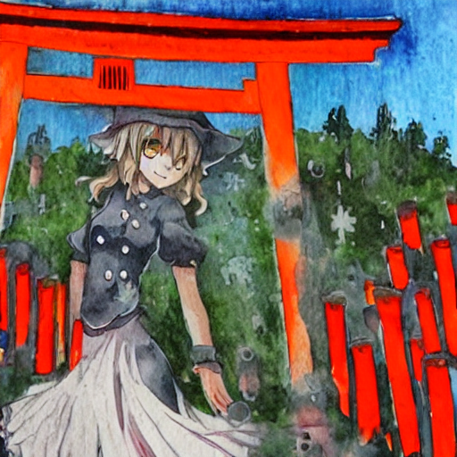
Denoising high sigmas with a background expert, mid/low sigmas with a character expert
eDiff-I shows us that an ensemble of expert denoisers can specialize in different parts of the denoising schedule. I wanted to try mixing a "scene specialist" and a "character" specialist, by swapping stable-diffusion checkpoint during the denoising process.
Twitter thread — Japanese stable-diffusion as scene expert, waifu-diffusion as character expert
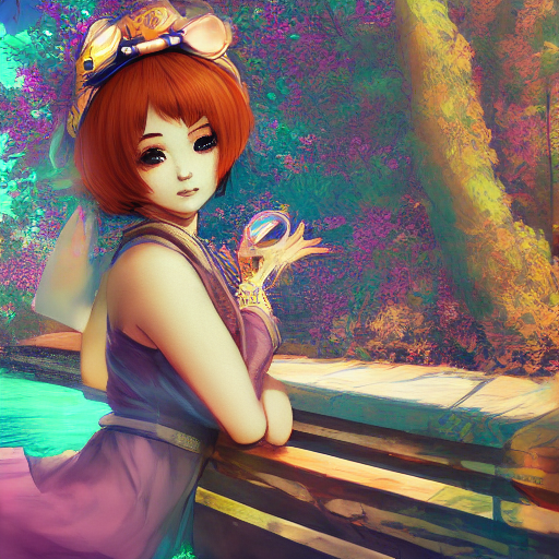
Twitter thread — SD2 as subject expert, waifu-diffusion as style expert
Inferencing from diffusion models is slow on Mac, so I was keen to cut down the number of steps required for sampling.
We can be tactical about which sigmas we denoise. We get good facial details by including a step at sigma ~0.1, and we can even end our denoising schedule there, rather than going all the way down to stable-diffusion's minimum of 0.0292. Raising sigma_min like this cuts a lot of low sigma steps out of our schedule, which doesn't seem to harm the image much; an 8-step schedule ending at sigma 0.0936 can often make good images with Heun sampler.
I managed some 4-step samples as well; hand-picked sigmas were able to get better results than the Karras schedule, by optimizing for the timesteps at which the Unet proved most effective.
I wonder whether the yield could be made more consistent by training an ensemble of expert denoisers, specialized at each of those 4 sigmas!
The pursuit for few-step sampling also included a collaboration with Katherine Crowson — she suggested to try modifying the DPM-Solver++(2M) sampler to begin with a DPM-Solver++(2S) step, to warm up the linear multistep. It seemed to help!
Fixing a smaller-than-usual image by subtracting representative attention scores from denominator
Stable-diffusion is poor at generating images smaller or larger than those in its training distribution. I wondered how much of that could be attributed to the impact of an unexpected key length on self-attention's softmax averaging.
My hypothesis was that if we could adjust the magnitude of the softmax denominator to be in-distribution: we may be able to correctly generate images at out-of-distribution sizes without retraining.
If our image is too small: our self-attention key length will be small, our softmax denominator will be small, our attention probabilities will be large. Vice-versa for "too large".
Can we bring a larger-than-usual image into distribution by computing softmax denominator from a subset of attention scores? Can we bring a smaller-than-usual image into distribution by extrapolating "more attention scores" in our denominator by sampling from those available?
This was a research collaboration I pursued with Kharr and tpapp157 at EleutherAI. I am currently writing up our findings, to publish as an EleutherAI blog post.
Fixing a larger-than-usual image by computing denominator from topk attention scores
When to skip CFG for speedup
Full CFG
Partial CFG
Skipping CFG for half the denoising schedule saves compute, and image looks similar
CFG isn't free. It doubles our batch size. Yet we rely on it for generating relevant images.
Do we need CFG for the entire denoising schedule though?
I hypothesize that we only need CFG for establishing the composition. Denoising a highly-noised image is a different problem (detail invention) to denoising a lightly-noised image (gap-filling). Perhaps a gap-filling problem is easy enough that we can make a correct denoising prediction without the help of CFG?
I found that we could turn off CFG for the second half of the denoising schedule (sigmas below 1.1), and get approximately the same picture. This sped up image generation by 21%, and is applicable to any diffusion model.
The reason it saves so much compute, is because it effectively halves the batch size for half of the denoising process.
I had originally hoped that for low-sigma denoising we could turn off both self-attention and cross-attention, and regard it as a gap-filling problem for convolutions to solve. I wasn't able to remove attention from stable-diffusion without adverse effect. But perhaps an ensemble of expert denoisers could include a fine-detail expert for low sigmas, which operates without attention (e.g. Paella).
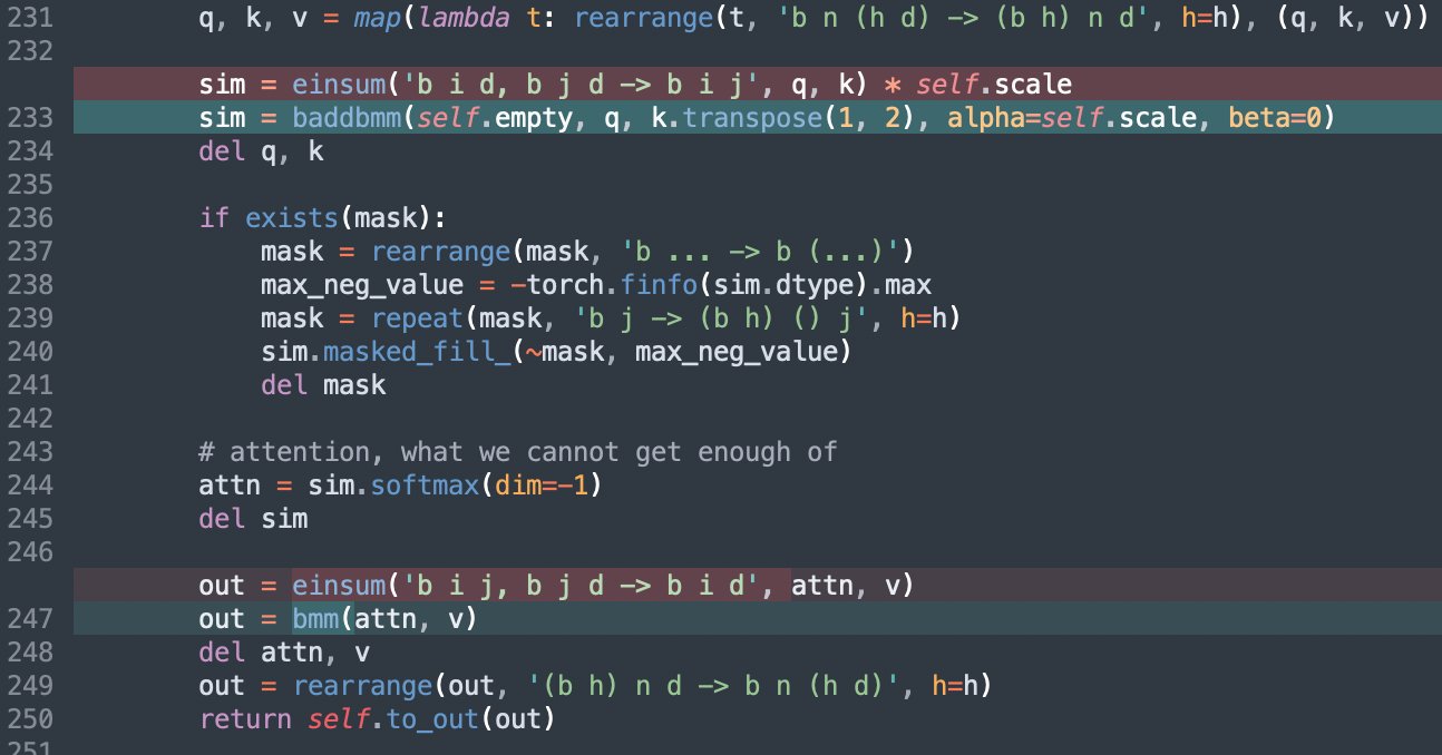
Thanks to Suraj Patil for showing how to reformulate the attention einsums as matmuls, and to Nouamane Tazi for showing how to fuse scale factors into matmuls.
The significance for CUDA users is lessened now that Flash Attention is widely available. But this remains a welcome speedup on Mac.
I sped up LLaMA_MPS by 4.7% with this same technique.
A float16 Unet is sufficient, so long as you sample in float32.
A float16 Unet can produce samples competitive with those from a float32 Unet. So long as we sample in float32.
Everything inside the Unet (except computing timestep embedding) can be float16. Everything outside (e.g. noised latents, k-diffusion sampling) should be float32.
PyTorch's MPS backend encounters tensor striding issues in all sorts of places
I started my machine learning journey on an M1 Max. The 64GB of unified memory is useful, but performance and software support are far away from what CUDA offers.
I've spent a lot of time debugging errors in the PyTorch MPS backend, and I try to report these and provide minimal repros as often as I can. In particular I was able to prevent a 42x einsum() performance regression from being included in the 1.13.0 release.
Frequently I am able to find workarounds (e.g. copying tensors, using different operations, falling back to CPU). The most common problems are with tensor-striding or indexing. Symptoms usually manifest as a black image, or one with a repeating grid pattern.
Backwards pass is a lot harder (issues include NaN loss or autograd crashes), but I got textual inversion working and CLIP guidance working despite that.
There is an optimization employed by PyTorch's torch.nn.MultiheadAttention, which has not made it into diffusers' or CompVis's attention implementations.
q_proj, k_proj and v_proj are computed separately. but if their weights were concatenated: it would be possible to perform q,k,v projections simultaneously for self-attention, or q and kv for cross-attention.
On M1 Max, this didn't result in any measurable difference. Mac performance varies a lot with system temperature, and there are not profiling tools for PyTorch MPS backend, which makes it hard to benchmark small phenomena.
I also played with reshaping q,k,v together in one operation, and eliminating the double-reshape of the key tensor. Once again: no measurable difference on Mac.
A fun thing you can do is eliminate the scale factor from the attention calculation entirely, by fusing it into the q,k projection weights. I got this idea from a footnote in One Write-Head is All You Need. I didn't measure any speed difference compared to fusing the scale into the baddbmm matmul though.
Attention — the revolutionary algorithm that ushered in the transformer era — relies on large matrix multiplications and softmax operations. Even a modest stable-diffusion image (512x512) can require self-attention buffers as large as 512MB, growing quadratically with sequence length.
Self-attention Does Not Need O(n²) Memory showed how to carve the matmul into chunks, and
produce the softmax denominator by accumulating per-chunk maxima rather than requiring all attention scores in-memory simultaneously.
Prior art existed, but I wished to add a few optimizations:
Twitter thread (demonstrating generation of a high-res image).
ToMe token merging
Facebook Research published ToMe token-merging, which reduces the memory/computation requirements of diffusion models by merging similar tokens together.
I collaborated with one of the authors (Daniel Bolya) and a GitHub contributor (lalalune) to get this technique working for CompVis stable-diffusion. The paper already had a preliminary stable-diffusion implementation, but it was not included in the initial release (as further evaluation was required).
There's now an official implementation, which applies the token merging earlier than where I did.
ToMe does result in lower fidelity, so I think it needs to be used judiciously.
I reckon it should be applied during early parts (e.g. sigma>1) of the denoising schedule (then disable it thereafter, to let remaining denoising steps fill in fine detail). It should only be used when you're pinched for compute — e.g. in the Unet blocks where the sequence length is largest.
ToMe may have an unexpected extra use: fixing softmax averaging when producing images larger than those in the training distribution. We can use it to diminish our self-attention key and value to an in-distribution sequence length.
I did not manage to reproduce the best results of the paper, but the author confirmed that my results may still be consistent with what they'd expect, and that my implementation could be correct.
I believe I found some mistakes in how the reference implementation splices structures together. The natural language processing that they use to split text prompts into noun-phrases (nltk+stanza), employs a different tokenizer than CLIP. In my implementation: I use regex to solve each noun-phrase's insertion point in the prompt.
My implementation also takes care to do more work in parallel, and especially optimizes attention.
Compiling stable-diffusion for CoreML was already a solved problem (thanks to initial investigations by contributors such as Matt Waller, Ollin Boer Bohan and the diffusers team), but getting it to schedule work on the Apple Neural Engine had not yet been achieved.
Based on Apple's whitepaper: I assumed that the reason the Neural Engine was unutilized, was because the tensor operations were not in the Neural Engine's preferred format.
The Unet was originally optimized for GPU, with 3D tensors in channels-last format ([Batch, Tokens, Channels]).
I changed each layer of diffusers' stable-diffusion Unet to use tensors in [Batch, Channels, 1, Tokens] format (4D, channels-first).
I had to make changes to the coremltools compiler (describe unsupported operations differently) to get it to compile the model.
I also tried compiling the sampler (which invokes the model) to CoreML, which required me to fix some bugs in coremltools.
Neural Engine only supports float16. Ordinarily, coremltools advises to trace the model in float32, and rely on their conversion to cast operations to float16 (and optimize the casts out).
I didn't want noisy casts in the IR code (since I was debugging the IR whenever the compiler had bugs), so I modified coremltools to prefer float16 as its default float type, and traced the Unet in float16 via MPS backend.
I managed to release before Apple did, but it turns out I was missing one crucial piece to target Neural Engine: I needed a macOS public beta. After Apple explained this in their release announcement, I was able to benchmark my model.
By default, k-diffusion's CompVis denoiser wrappers do not discretize the sigma schedule. I didn't know about that convenient boolean! So I tried to fix this the hard way, and found something interesting along the way.
I compared k-diffusion's sample_heun code with the algorithm from the EDM paper, and further scrutinized it against the "iDDPM practical considerations" from section C.3.4 of said paper.
I found that the sigma_hat parameter was not being discretized (even when quantize=True was enabled). This means that the Unet may be asked to denoise a sigma outside of the discrete sigmas in its training distribution.
This parameter is only referenced when churn is enabled, so the damage is minimal. I still haven't seen anybody play with churn, but it's a parameter which injects noise; I believe the effect should be similar to the "creativity" with which euler_ancestral is credited.
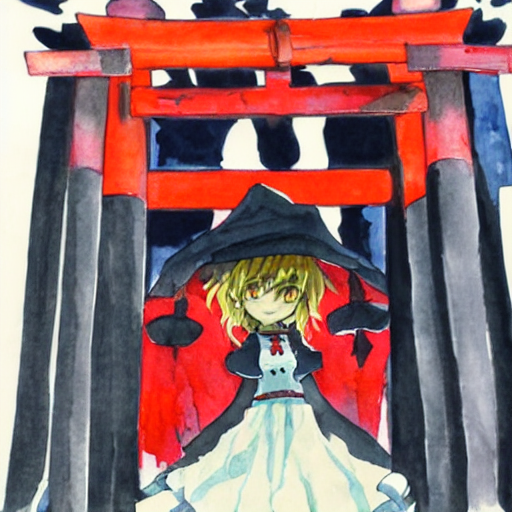
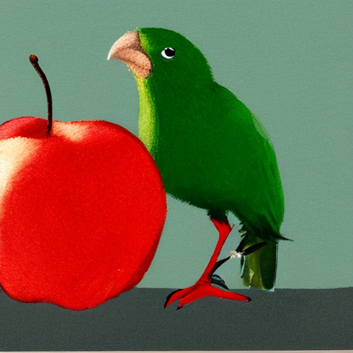
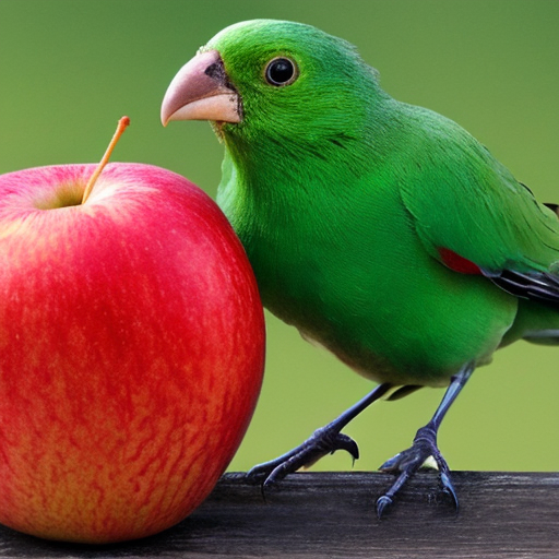
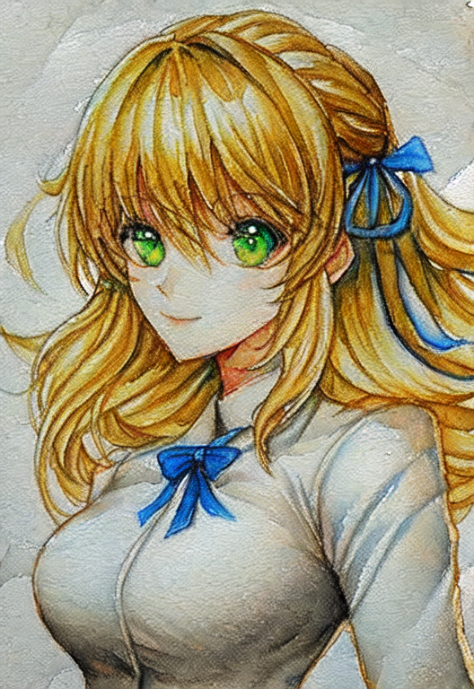
Diffusion models can use a text condition for generating an image. How would we transition between two conditions?
Stable-diffusion is conditioned on CLIP text embeddings: sequences of word embeddings. Similar concepts are embedded to similar locations in space. Consequently, by interpolating between word embedding coordinates we can do a semantic transition between concepts.
CLIP word embeddings have positions in a many-dimensional (e.g. 768) hyperspace. They are Gaussian-distributed, so we can treat them as points on a unit hypersphere. Thus the correct way to interpolate between them is with a spherical (as opposed to linear) interpolation.
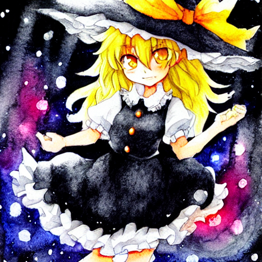
Special thanks to Cafe from the Touhou Project AI Discord for sponsoring this open-source research (long animations became possible thanks to new hardware).
A particular challenge was getting it to work on Mac. Reducing the batch size (by disabling CFG) fixed it.
I later found that CFG could be enabled, so long as the cond and uncond were submitted to the Unet in separate batches.
Thanks to Matt Waller for sharing the tip of single-cond batches on Mac, who found the same trick fixed bugs in early CoreML models.
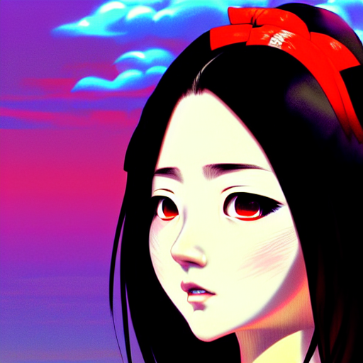
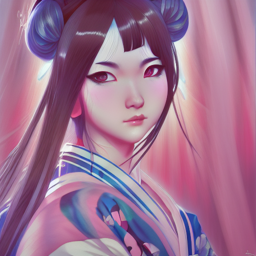
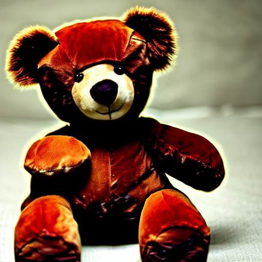
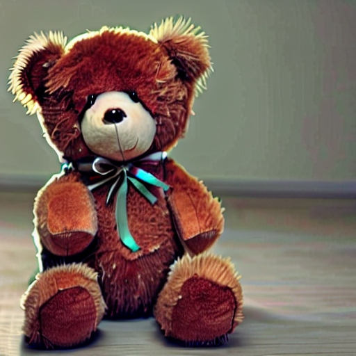
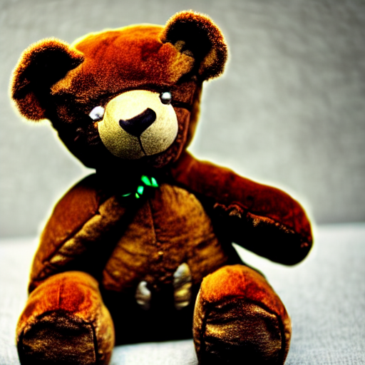
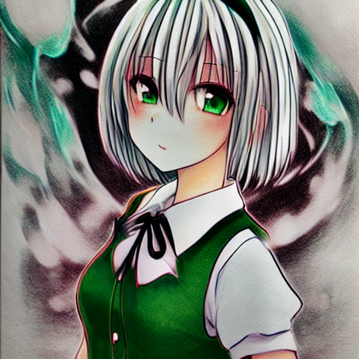
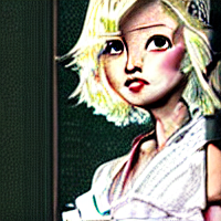
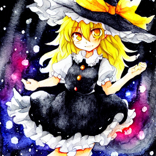
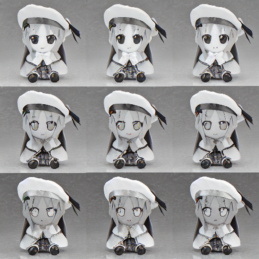
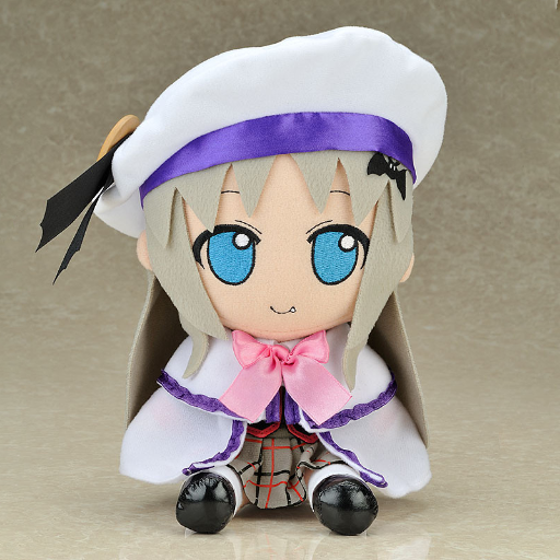
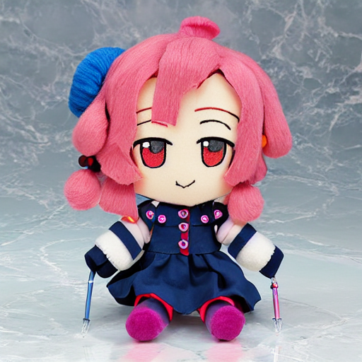
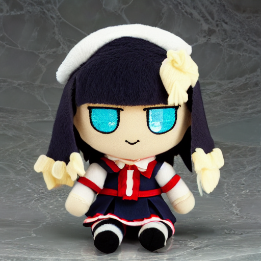
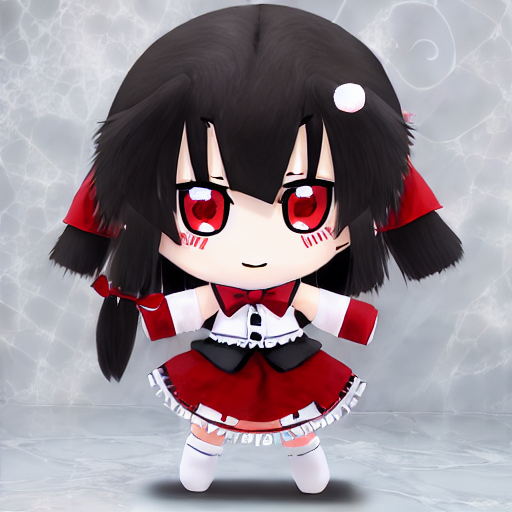
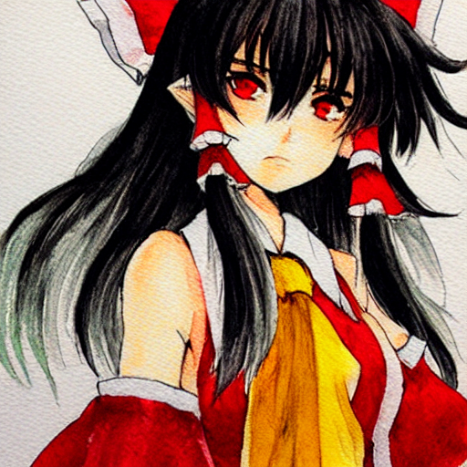
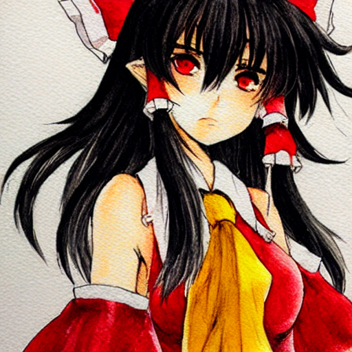
It's interesting how the semantic that Textual Inversion learns from a fumo plushie (big head, stubby limbs) works even in stable-diffusion checkpoints which forgot the photoreal style. The result is a graphic very similar to a chibi illustration.
A non-photoreal checkpoint generates fumos as chibis
Attention masking
Usual
BOS+EOS only
Masking out all word embeddings except for BOS and EOS
Attention supports an optional bias parameter. Most often, it's used as a mask (applying a highly negative bias to attention scores at given indices). The mask can (e.g. in language models) be a "causal" mask (hide future information in the sequence). It can also be used to hide padding tokens when data of varying sequence lengths have to coexist in the same batch.
I wondered what would happen if we conditioned stable-diffusion on a CLIP embedding with most of its tokens masked-out. Structured Diffusion explains that the "high-level semantic" of a text prompt gets pooled into the CLIP EOS word embedding.
If we mask out every word embedding except for EOS: would it look similar to the unmasked condition?
Turns out yes: a lot of the semantic survives. You need to keep the BOS embedding also (every condition in stable-diffusion's training set has the same BOS, so hiding it throws the inference out-of-distribution).
Increasing step count with and without Brownian tree noise sampling
One problem with few-step sampling is that after you find an image that has potential: you may find that it completely changes if you master with more steps. This is why we could want stable convergence (the idea that image structure won't change drastically during the denoising process).
Katherine Crowson added Brownian Tree noise sampling to k-diffusion. I evaluated it, and found that it succeeded in giving a 10-step sample the same high-level composition as a 100-step (i.e. converged) sample.
I further evaluated how to achieve comparable results with adaptive samplers (e.g. which seek to give you a convergence guarantee). Raising eta to 0.75 and reducing rtol to 0.025 seemed to help, but I didn't manage to convince myself I'd found a dependable configuration.
Reducing rho to allocate more high sigmas (>2), fixes clothing
When few-step sampling, you may find that your image is moreorless good, but has some errors in fine detail or composition.
You can change the rho parameter of a Karras schedule to bend the denoising schedule to allocate more sigmas to the highly-noised or lightly-noised part of the schedule.
rho is typically 7, but decreasing it (e.g. to 5) will sample more from high sigmas (>2), expending more effort on high-level composition.
Conversely: increasing it (e.g. to 10) will sample more from low sigmas (<1), expending more effort on fine detail.
When it comes to representation of floating-point numbers: neural networks are far more sensitive to the size of the exponent than the mantissa.
There is an interesting property of the floating-point exponent: exponents can be multiplied by other exponents cheaply (integer addition). This present an opportunity to compute the exponent portion of a matrix multiplication without using any floating-point hardware.
I decomposed a matrix into its mantissa and exponent, multiplied its separate parts (the mantissae multiply via Hadamard product, the exponents multiply via addition), then recombined them to verify that it yields the same result as regular matrix multiplication.
This is just step 1 of a larger idea.
My hope is that we could discard the mantissa entirely, for parts of a neural network that primarily care about magnitude (e.g. computing attention probabilities in scaled dot product attention).
I think some extra tricks would be needed to make exponent-only attention probabilities differentiable. But if there's a way to do this, then it could drastically reduce the amount of silicon required for transformer training.
If it cannot be differentiated: exponent-only attention probabilities could still be useful for optimizing inference.
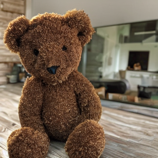
I made some animations to illustrate how stable-diffusion's denoising process works. We can use k-diffusion's callback to log intermediate latents from each sampling step.
At first I visualized this via stable-diffusion's VAE. But noised latents are outside of its training distribution, so I wanted to do a simpler decode (just a colour-space conversion) to avoid inventing detail or upsampling. So for my second attempt I used my approximate decoder.
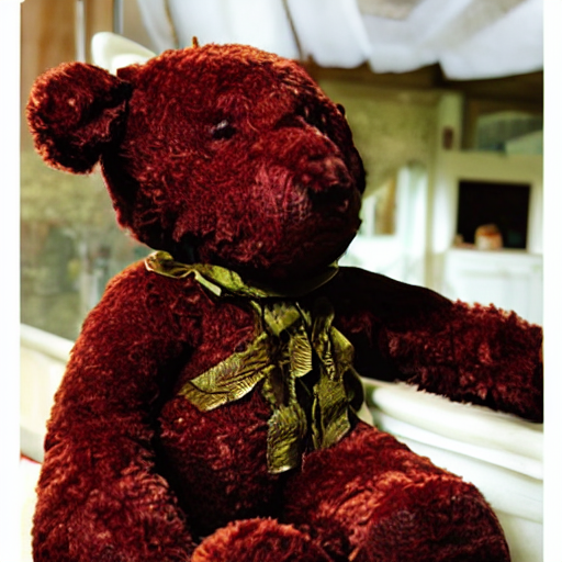
I made some animations to illustrate the effect of classifier-free guidance on stable-diffusion's output (i.e. making denoising predictions more relevant to text condition).
See also my dynamic thresholding techniques for how to prevent clipping at high CFG scales.
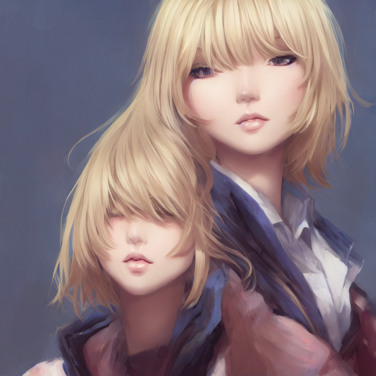
Image different but still coherent after dropping a value head
I was discussing One Write-Head is All You Need with Aditya Ramesh (OpenAI), who explained that diffusion models sometimes learn to drop out attention heads.
I wondered whether stable-diffusion was doing this. If that were the case: perhaps we could verify it by replacing an attention head's weights with weights copied from one of its siblings. If this did not result in any change: perhaps it would indicate that the attention head wasn't being used.
Depending on how many/which heads I dropped out: I found that it didn't completely destroy the image. In some cases I still got a perfectly usable image.
I'd love to see a large-scale model evaluate the One Write-Head paper. It's a bit harder now that we're accustomed to Flash Attention - a bespoke CUDA kernel or Triton implementation would need to be created to get performance parity.